Fundamental Concepts in Markov Decision Process and Reinforcement Learning

MDP is a way to model the world dynamics. We have an agent in an environment and we want the agent to interact with the environment in a desired manner. The following image illustrates the environment setup of RL and MDP.

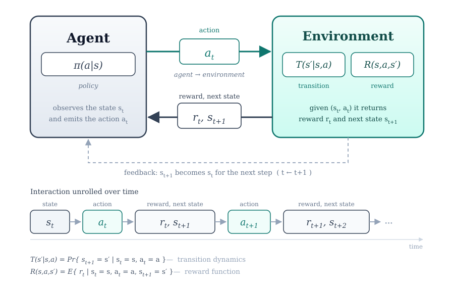
The agent observes the current world state \(s_{t}\), and performs an action \(a_{t}\) based on the state observed and a policy \(\pi(a|s)\), which basically tells which action to perform at some state. Moreover, the policy is usually stochastic, meaning the policy \(\pi(a|s)\) is a distribution over action space \(A\) conditioned by state \(s_{t}\).

The environment is also stochastic. Given the current world state and what the agent has done (i.e., the state and action), the world changes correspondingly. The world state of time \(t+1\) is sampled from the distribution \(T(s'|s,a)\), called transition. Besides world transition, we also have a reward function \(R(s,a,s')\) that judges whether this action is good or not.

Trajectory

In MDP/RL settings, we usually called an alternating sequence of \(s,a,r\) a trajectory, denoted by \(\tau\):

\[ \tau = (s_{0},a_{0},r_{0},s_{1},a_{1},r_{1},\dots) \]

To measure the “goodness” of a trajectory, we can just accumulate the rewards. We also introduce discounting here, because intuitively, we should encourage early beneficial actions. We call this discounting cumulative rewards \(G_{t}\). The subscript means, we start from step \(t\).

\[ G_{t} = \sum_{k=0}^{\infin} \gamma^{k} r_{t+k} \]

The state value of \(s_{t}\) refers to the expected reward \(G_{t}\) starting from it and we perform according to the policy \(\pi\) (we are computing expectation over the distribution of the action space)

\[ V^{\pi}(s_{t}) = \mathbb{E}_{\pi} \left[ G_{t} | S_{t}=s_{t} \right] \]

The action value of a state-action pair (called Q-state) \((s_{t},a_{t})\) refers to thet expected reward \(G_{t}\) starting from \(s_{t}\) and our first action is \(a_{t}\), and then we perform according to the policy \(\pi\).

\[ Q^{\pi}(s_{t},a_{t}) = \mathbb{E}_{\pi} \left[ G_{t} | S_{t}=s_{t}, A_{t}=a_{t} \right] \]

In some cases, when the reward function is mal-defined, e.g., whatever action results in a positive reward, the discounted cumulative reward \(G_{t}\) is always positive. This will lead to some trouble during training (any action will be encouraged, because the reward is positive, causing the training unstable). Therefore, we use advantage to describe the extent to which an action is better than the average (the expectation).

\[ A^{\pi}(s,a) = Q^{\pi}(s,a) - V^{\pi}(s) \]

From the definition of state value and action value, we can infer their relationship.

\[\begin{aligned} V^{\pi}(s) &= \sum_{a} \pi(a|s) Q^{\pi}(s,a) \newline Q^{\pi}(s,a) &= \sum_{s'} T(s'|s,a) \left[ R(s,a,s') + \gamma V^{\pi}(s') \right] \end{aligned}\]

By plugging \(Q^{\pi}, V^{\pi}\) back into equations, we can get the Bellman Equation.

\begin{equation} \boxed{ \begin{split} V^{\pi}(s) &= \sum_{a} \pi(a|s) \sum_{s'} T(s'|s,a) \left[ R(s,a,s') + \gamma V^{\pi}(s') \right] \\ Q^{\pi}(s,a) &= \sum_{s'} T(s'|s,a) \left[ R(s,a,s') + \gamma \sum_{a} \pi(a|s) Q^{\pi}(s,a) \right] \end{split} } \end{equation}

Let’s call the policy that is used to generate trajectories behaviour policy \(\mu\) and the policy that is to be optimized target policy \(\pi\). On-policy means that these two policies are the same, i.e., \(\mu=\pi\), we’re using our data to train ourselves. In contrast, off-policy means that these two policies are not the same, \(\mu \ne \pi\), we’re using data generated by others to train our policy.